Solidworks Simulation Benchmarks (for Real Studies) – 2022 Edition

It’s been a while since we ran new benchmarks on simulation problems. It also took Intel a well-documented long time to get a new architecture and process on the market. After many hours checking new processor release dates and rumored specs, while waiting on studies to run, we finally got a new desktop system. We were holding out for a “4th Generation Xeon Scalable” rig, but settled on a “12th Generation Core” system at an attractive price.

High level specs on this new box include an Intel Core i7-12700k processor, 2 TB NVMe main drive, nVidia RTX 3080 graphics, and 128 GB of DDR5 memory. After setup and a quick stress test benchmarks were the first order of business. Again standard Passmark tests were run and then the same sim models we ran in Solidworks 2018 were run in Solidworks 2020.

The old benchmark article, from December 2018, can be found here.

Subject systems still available to bang on are the 6th generation 6700K, a 9th generation 9800X, and of course the new 12700K. The basic specs and synthetic benchmark results are tabulated below.

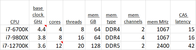
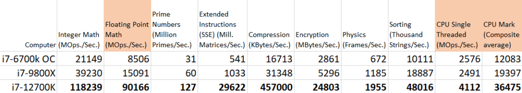
The 12th generation chip, finally made on a true 10 nm process, shows a great leap in raw performance. Gritty details can be found all over the internet about the details of the new chip. We noted that they took advantage of the smaller process to pack larger local caches into the die. High level Intel documents talk about added cleverness in ordering and streamlining operations. Busses to memory and storage are faster and wider. Then there’s the whole P-core and E-core hybrid design added to the system.

But the real test of all that brute power and cleverness is in performance on real problems. So we return to the same problems as before.

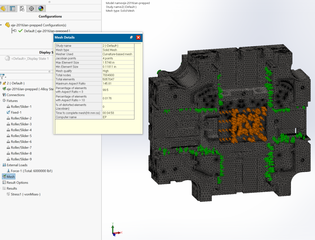
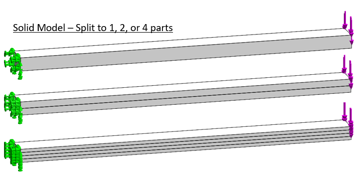
This large solid block with lots of internal detail is used to check mesh speed and solve time with an iterative solver.

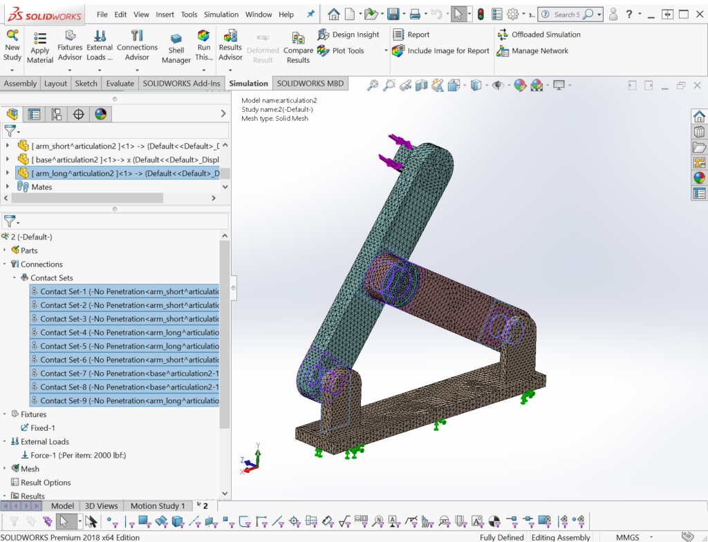
This artificial test problem is used to test run time with contacts in a direct solver.

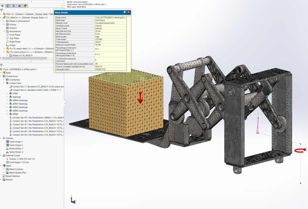
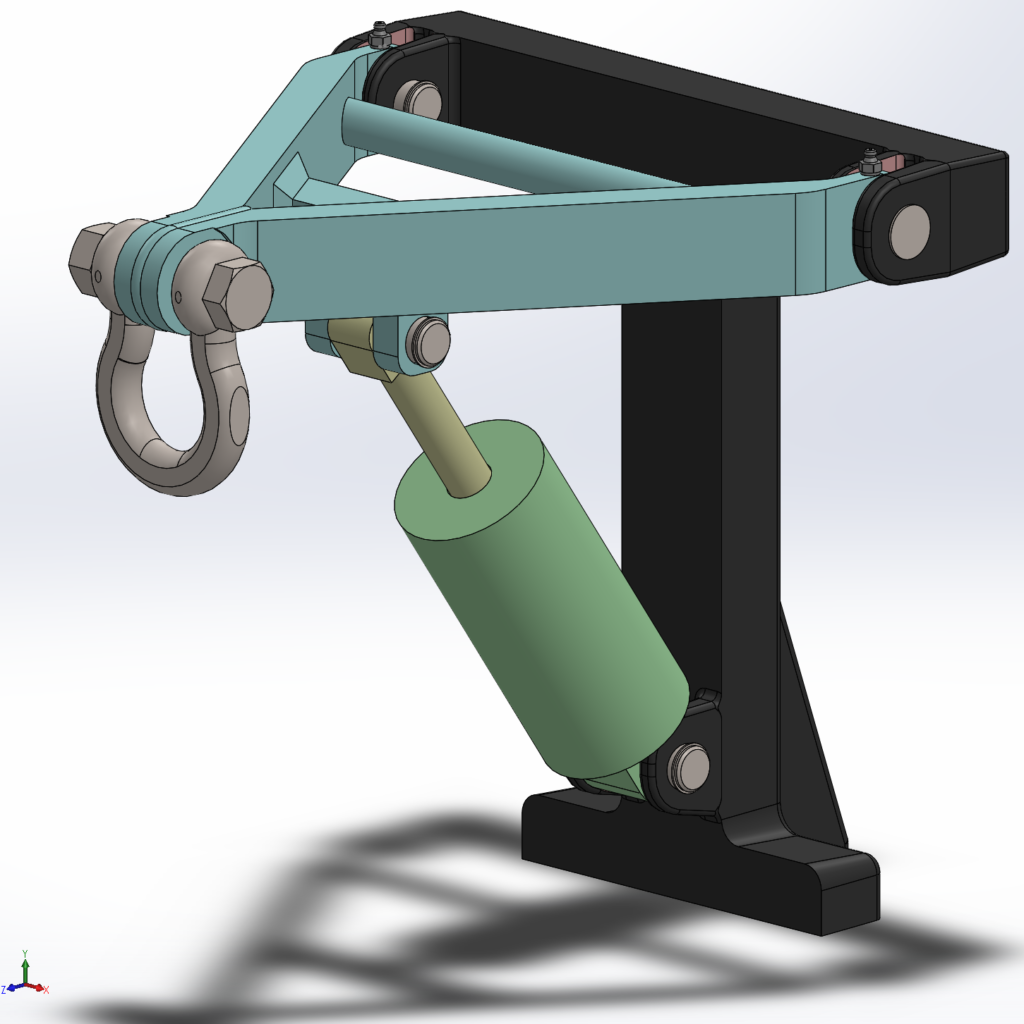
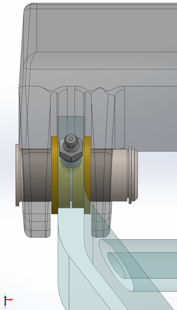
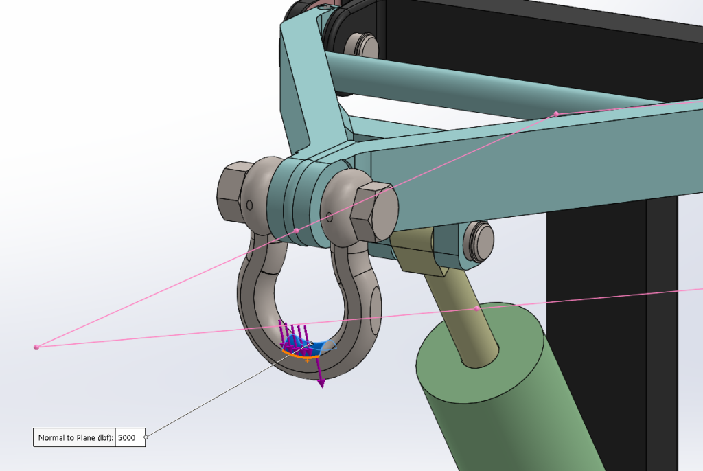
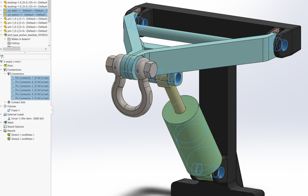
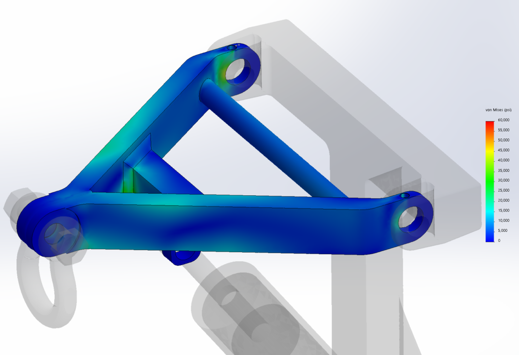
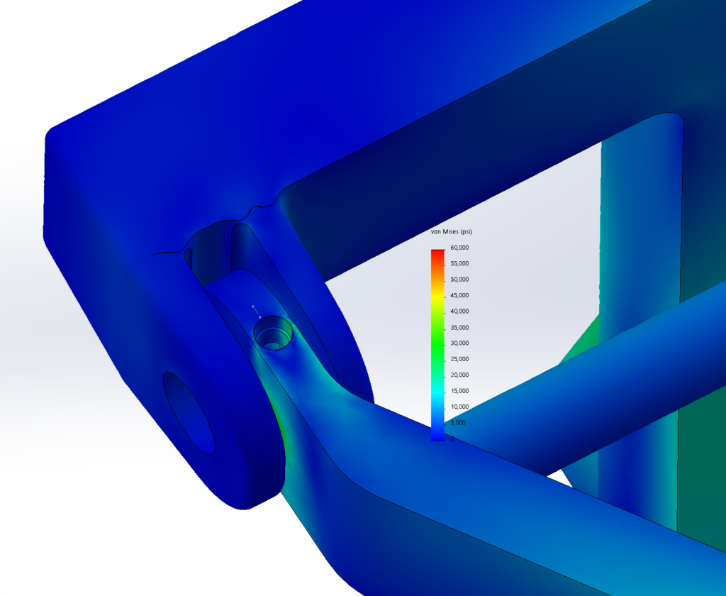
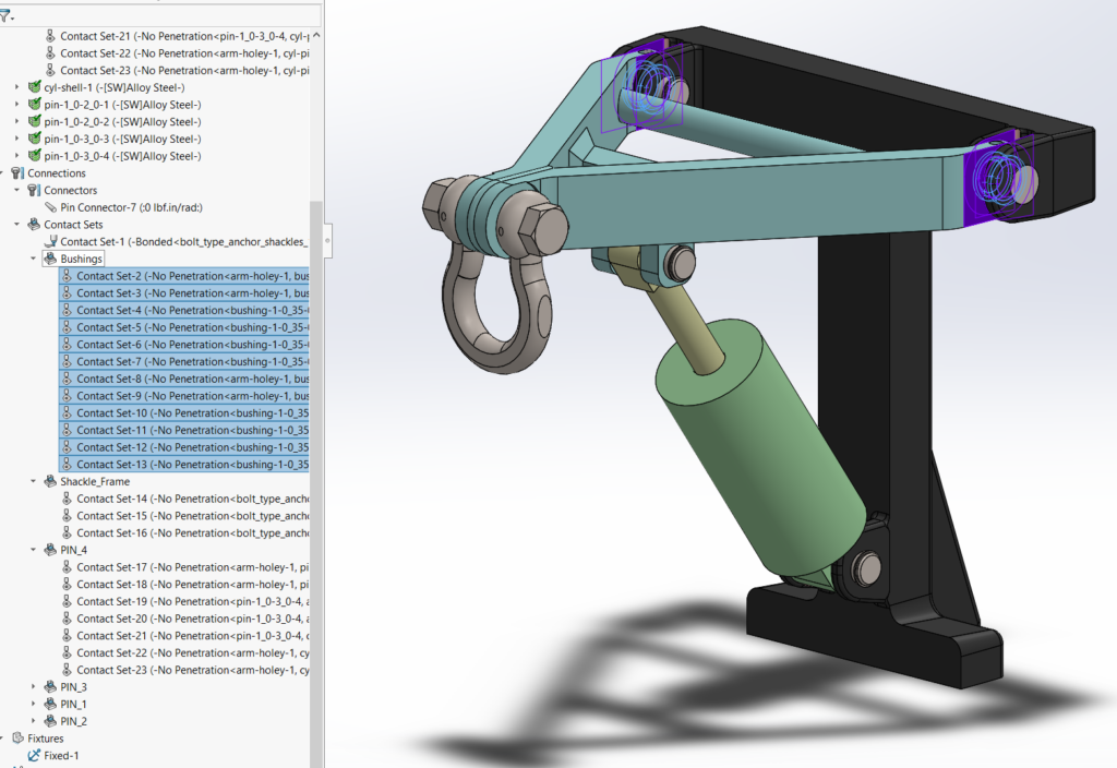
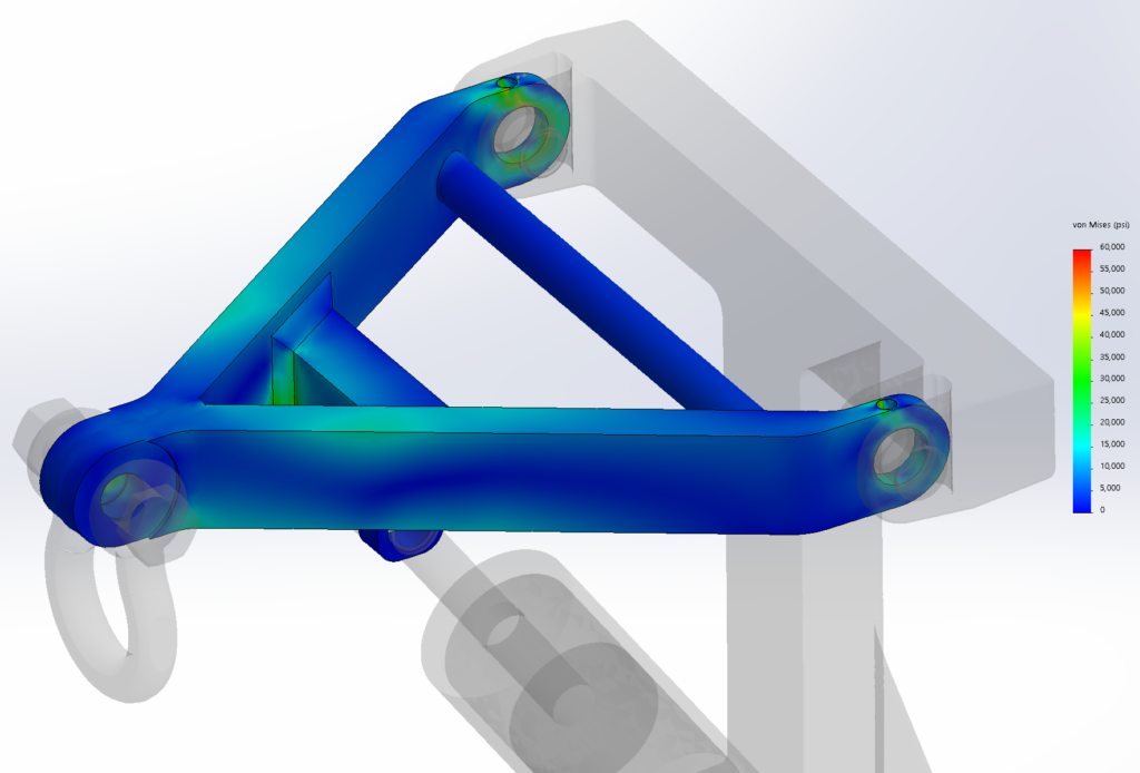
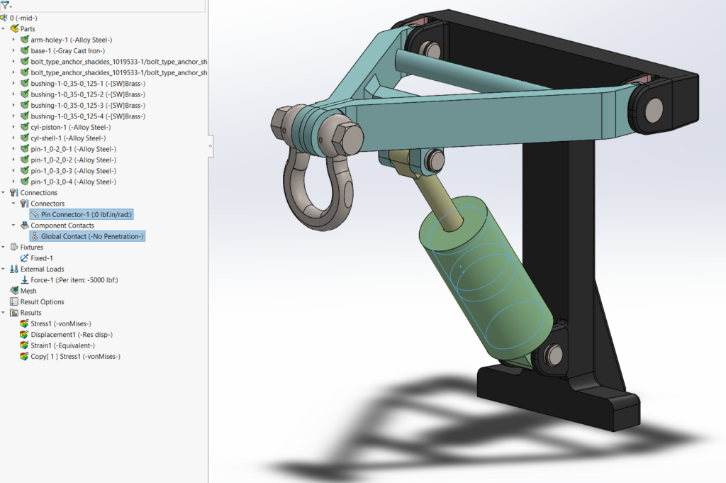
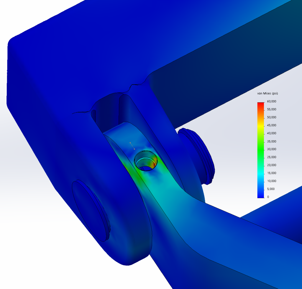
This reach-lift assembly, with an overly fine mesh, gives us the longest run times, with lots of contact and connectors.

The Solidworks Simulation 2020 results are first compared to the available results from 2018.

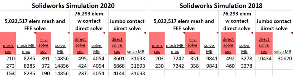
We note that Solidworks 2020 uses a bit more RAM for each operation, we assume in a trade-off for calculation speed. This is reasonable with memory prices dropping logarithmically through recent years (though at this writing DDR5 is still a bit precious).

The processor models aren’t labeled on that table, but one can readily guess that the bottom line is the 12700K. We are very impressed with the results. Solve times are basically halved, using an inexpensive mainstream processor. To visualize this here are more traditional benchmark charts.

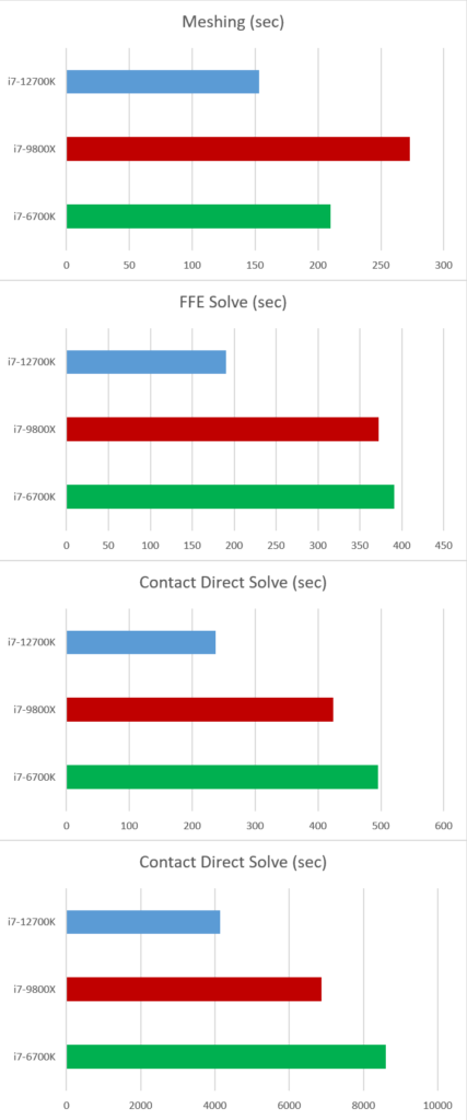
Run times are getting faster, and this is a problem! Our production analyses are getting down to where there isn’t even time to go get a cup of coffee or catch up on important forum posts.

In all seriousness, we’re used to having time to look over new results and integrate them into a running report, possibly discussing updates with a client, before the next iteration runs. We’ll have to work on a new scheme of time management, and throw a bone to the dog who used to get played with more while the computer cranked.

[Notably absent here are results for AMD systems and newer version of Solidworks. We’re still an Intel shop, as other testers have found the AMD architectures poor for Solidworks mechanical sim, though those tests are dated. Solidworks 2021 posed new challenges, with badly documented changes in the interface and some apparent bugs that Dassault has not resolved with us, and we just haven’t tried 2022 yet. If anyone wants to try it, the smaller direct solve study is available here. We’d be happy to see new results.]

Mesh Density Challenge 2 of 2

In the previous piece we looked at beam bending with solid and hollow sections, with different numbers of elements across the body or the wall thickness. Here we switch from bending to torsion. In torsion open shapes behave very different from closed sections.

By closed section we mean something like the cylinder below. The section is made “open” by cutting a lengthwise slot through the entire length [the classic example for this is to take a whole toilet paper tube then cutting it once and seeing the difference in twisting stiffness].

The cylinder is fixed on the left end. A pure torque is applied to the right end face. The second shape shows the slot cut and a split which cuts the shape into two bodies.

Again we mesh the body first with linear elements, then second order elements. The body is split to force multiple elements through the thickness at the same mesh settings. Since a closed cylinder is very efficient in torsion displacements are very small and we won’t plot displacement here.

Results on the cut cylinder follow. Even with coarse linear elements the result looks realistic.

But when we use high quality mesh the body is much more flexible. Stress predictions also change significantly. The extremely fine mesh result is our reference.

Tabulation of results shows again that the use of second-order elements goes a long way toward delivering ideal results.

The engineer knows that asymmetric open sections are very poor in torsion, but sometimes that loading has to be borne. A simple C-channel is modeled and split into two or four bodies.

The setup has the left end fully constrained again. The right end has a moment applied by opposing forces along the top and bottom edges.

Stress results follow a now familiar pattern. With a coarse linear mesh the stress pattern is ‘lumpy’ and the deflection is very low.

Viewed end-on the relative deflection is readily compared.

Twist of the high quality meshes is much greater at any density.

The tabulation shows the advantage of the “high-quality” mesh. In this case the mesh density needs more than two elements across the thickness to bring good results.

In conclusion we find that relatively coarse solid meshes with second-order elements usually provide good results in Solidworks Simulation. Relative importance of mesh density varies with local loading conditions. It is advisable to run mesh sensitivity studies, at least on any new class of problem. Our usual practice is to get what we think is a good result, then near then end of the project bump up the mesh density on one study to the maximum practical mesh size. After a long (maybe overnight) run, the results are compared to check that there is not a large divergence.

Mesh Density Challenge 1 of 2

The claim comes up often when a FEA result is presented, “You need to have multiple elements across that wall!” Well, do you? It may be important to good simulation results. We’ll look here at when it matters and how modern tools can put us at ease.

The “when it matters” is a questions of both application and point in history. Some readers will remember the ‘dark ages’ of manually generating finite element meshes in Hypermesh on a 16 megabyte workstation, setting up command line batch runs that ran overnight and took all day to visualize. In those days computer memory and compute cycles were precious. Nodes and elements, usually linear, had to be placed efficiently or human and machine resources were overtaxed or tied up for overly long. Today computer resources are vastly cheaper while human time is ever more precious.

The “when it matters” of application depends on the geometry and loading. The purpose of a dense mesh is to capture important gradients in a solution. In structural problems we’re looking primarily at stress gradients and total displacements. In “boring” areas of nearly constant stress, coarse meshes are adequate. Good displacement results may require finer meshes even over smooth stress fields.

Here we will look at bending problems, starting with a simple solid bar. It is fixed on the left and loaded vertically on the right, a textbook cantilever.

This bar is split two or four times to force mesh refinement across the bending thickness. For reference an extremely fine mesh is also put on the body.

Deformed stress results are shown for meshes with linear elements. Total deflection clearly increases with mesh density, as the stress field becomes smooth.

The same setups are run with Solidworks’ default “high quality” elements. Even with no refinement deflection is near as expected and the stress pattern is reasonable [stress color scales are all auto-scaled].

We can quickly discuss the issues here. With one element across the thickness, each tetrahedral element has one three-node face in tension or compression, and the opposite single-node vertex loaded the opposite direction.

Adjacent elements are loaded in opposite orientations. While the solver author has options in difference calculations (node centered vs. volume centered, etc), linear elements simply cannot resolve the stress gradients here. And if the base of one element is swelling next to the peak of another that is shrinking, that is another conundrum for the solver. It should be clear why tetrahedral elements especially are known for being “too stiff”. Rectangular brick elements would be better, but still cannot truly bend in one layer across the thickness of a beam.

The results are summarized below. “ref vm” is the probed stress; “max dy” is deflection at the cantilever tip. The last stress plots show the typical stress probe location, and illustrate ‘lumpiness’ in the stress result with linear versus second-order elements.

Taking the extremely fine result as reference, the coarse linear mesh badly under predicts stress and deflection. Switching to second-order elements immediately improves the result. Doubling and quadrupling the mesh size barely affects the stress results and just nudges the total deflection. But if we stick with the linear elements progress toward a smooth and flexible solution is painfully slow.

If bending is the primary load, an engineer will consider a shape like an I-beam. Here we have a simple beam with the flanges solid or split. We will repeat the meshing exercise, linear and second-order elements generated at different densities across the flanges.


Right away we should realize a difference from the coarse mesh solid bar. Even with the coarsest mesh, the elements loaded in tension are separate from those loaded in compression.

Now the linear element meshes all perform in a realistic way.

Response of the higher quality meshes can be differentiated in the numbers.

In compound or unknown loading, a closed section is the best choice. For comparison we will stick with a bending load and split the top and bottom faces.

Again the stretched and compressed faces are separated so linear elements give reasonable looking results.

With high quality elements the body is a little more flexible.

The stress results are pretty good even for the coarse draft mesh. The high quality mesh gives good displacement results even from the coarsest version.

What does this mean for the modern user? A mainstream workstation can solve multi-million element structural problems in main memory, and we often use direct solvers in Solidworks to breeze through 800,000 element setups in minutes. User time is much more valuable than computer time. We generally encourage people to stick with solid meshes and let the element count run up.

The challenge remains when long or thin portions of components are included. On high aspect ratio parts the element count can get extreme and Solidworks still does not give us tools to handle these sections efficiently. But we demonstrated here that coarse solid meshes on these “boring” connector sections can give usable results. Solidworks developers did us a huge favor by settling on the second order tetrahedral element, maximizing flexibility while retaining ease of fast automatic meshing. The user should focus mesh refinement on areas of detail and structural interest, like weld joints and contact interfaces.

In these studies we looked only at bending problems. There’s reason to wonder it torsion of long members might work differently. So we look at that in part two.
https://www.stonelakeanalytics.com/2020/11/09/mesh-density-challenge-2-of-2/

Connector or Crutch?

Most FEA tools have a toolbox of handy features one can use to simulate mechanical elements. When not all the hardware in an assembly is modeled, or modeled badly, or modeled such that it makes interferences that must be resolved, these tools are as handy as a big hammer when the manual says “slip fit”.

We use a great many of the “pin” connector in Solidworks Simulation. Where holes (and/or shafts) are meant to be aligned or a body is supposed to have free rotation* it’s just a couple clicks to get the relationship established in Sim. Forces are transmitted cleanly and system response can be predicted well. But there is a catch – nodes on the hole or shaft walls are locked into relative position on the original theoretical cylinder. This has implications, locally at least.

[* in Solidworks 2018 the pin connector tool was improved to allow selection of more than two cylindrical surfaces, but free-rotation of the bodies was broken; a fix is promised for 2020.]

The following story is illustrated on a bespoke model, but inspired by a real story from a client who has some broken parts.

A small lift is modeled. A hydraulic cylinder raises and lowers an A-frame which has a shackle installed on the pointed end. The cylinder shell and the wide ends of the A-frame mount to a solid casting by pins through double-clevis joints. The assembly is about 18 inches tall with a 14 inch reach.

Most of the pin connections are plain bearings, and fairly loose. But it was decided that the rear joints of the A-frame should be tight, have brass bushings, and be greaseable. So the bore through the A-frame arms is larger, and there is a cross-drilled hole for a threaded grease fitting.

The customer wants to lift a two ton load, which is known to swing some. For our studies a 5000 lbf force is used, angled a bit to the right.

All the hardware came in the model, accurate (yay), not-overly-detailed (bonus), centered (wow), and close-fitting (excellent for contact analysis). But the fastest way to set it up is to exclude all the hardware and use the trusty pin connector.

The modeled pins and pin-bushing sets are replaced by single pin connectors. Only the shackle remains, but it also is connected to the A-frame by a pin connector. (Another pin connector holds relative position of the cylinder halves.)

Since everything is connected by rigid “pins”, the FEA solution is practically a static solve of a single solid body. It runs in 24 seconds.

Stresses in the wrought steel frame look pretty good. But what about that grease fitting hole? It left some pretty thin walls. Some mesh refinement was put around here and a closer look taken.

Ok, the thin walls are working hard, but it still looks good enough. Since it runs fast, we can set up runs with the cylinder at all different strokes to see what happens, generate all kinds of force data, and keep the customer happy. …Until something breaks and they want to know why.

Setting up this problem the hard way, i.e. the right way, means ditching most of the pin connectors and using the supplied hardware (or custom modeling simple hardware to do the job in Sim).

Over 40 high-accuracy no-penetration contact pairs are manually defined. At every joint each part is in contact on a cylinder and two lateral faces. Only the cylinder’s pin connector remains.

The stress pattern is very different in the mounting ears. Elevated stress is seen all the way around the joint, whereas on the first run it was only on the load side.

Now the full stress concentration from the drilled hole is captured. Further study can show how the stress might be sensitive to dimensional variance, like the hole being off-center.

At what cost did we get the better answer? It took about 20 minutes to set up all those contacts, and 25 minutes to run the study, versus a few minutes and 24 seconds to run the all-pin study. It beats getting a phone call from an angry end user who’s standing over a hole in the ground, made by some expensive equipment that just got dropped.

Incidentally, while all the setup work was going on, another easy-setup study was running.

Since it looked like the geometry was clean and complete, on starting Sim the simplest possible study was started. A single input of global no-penetration contact is used in place of pretty much everything else. This is almost always worth a try. It can take a lot of computer memory, and sometimes a long run time, but this study can run while all the other human work is being done on the ‘real’ setup.

In this case the quick-and-coarse study found the hot spot. With a couple mesh refinements it should match the answer in the full-manual-contact study. And it ran in under 13 minutes, quick enough that it could have guided all the later work.

Features like pin connectors are great, but the analyst has to understand what effect they have on the local situation.